Benchmarks

Introduction

Selecting the correct outlier detection and thresholding method can be a difficult task. Especially with all the different methods available in both stages. Quantifying how well each method performs over a variety of datasets may help when selecting based on either accuracy or robustness or both. PyOD provides a highly detailed analysis on the performance of all the available methods, with great insight and interpretability anomaly detection benchmark paper.

Since the thresholding methods are dependant on both the dataset and the outlier detection likelihood scores, in order to quantify how well a threshold method works, it must be tested against multiple datasets applying multiple outlier detection methods to each dataset. All the benchmark datasets can be found at ODDS.

To quantify how well the threshold method is able to correctly set inlier/outlier labels for a dataset, a well-defined metric must be used. The Matthews correlation coefficient (MCC) will be used as it provides a balanced measure when assessing class labels from a binary setup for an imbalanced dataset. This coefficient is given as,

$MCC = \frac{TP \cdot TN - FP \cdot FN}{\sqrt{(TP + FP) \cdot (TP + FN) \cdot (TN + FP) \cdot (TN + FN)}} \mathrm{,}$

where $TP, TN, FP, FN$ represent the true positive, true negative, false positive, and the false negative respectively. The MCC ranges from -1 to 1 where 1 represents a perfect prediction, 0 an average random prediction, and -1 an inverse prediction. This metric performs particularly well at providing a balanced score and penalizing thresholding methods that tend to over predict the best contamination level (most $TP$ and $TN$ and least $FP$ and $FN$ ) based on the selected outlier detection likelihood scores unlike the F1 score which focuses only on outliers. However, if finding and removing all the outliers regardless of how many inliers also get removed the F1 score is a better metric.

Since the thresholding method is heavily dependant on the outlier detection likelihood scores, and therefore the selected outlier detection method, simply calculating the MCC for each dataset would yield varying results that would have more dependance on the selected outlier method than the thresholding method. To correctly evaluate and eliminate the effects of the selected outlier detection method, the MCC deterioration will be used. This deterioration score is the difference between the MCC of the thresholded labels and the MCC for the labels produced by setting the true contamination level for the selected outlier detection method (e.g. KNN(contamination=true_contam)).

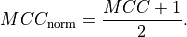
For consistency, the benchmark results below used the unit-normalized MCC, which is given by,

$MCC_{\rm{norm}} = \frac{MCC + 1}{2} \mathrm{.}$

Benchmarking

All the thresholders using default parameters were tested on the arrhythmia, cardio, glass, ionosphere, letter, lympho, mnist, musk, optdigits, pendigits, pima, satellite, satimage-2, vertebral, vowels, and wbc datasets using the PCA, MCD, KNN, IForest, GMM, and COPOD outlier methods on each dataset. The MCC deterioration was calculated for each instance and the mean and standard deviation of all the scores were calculated.

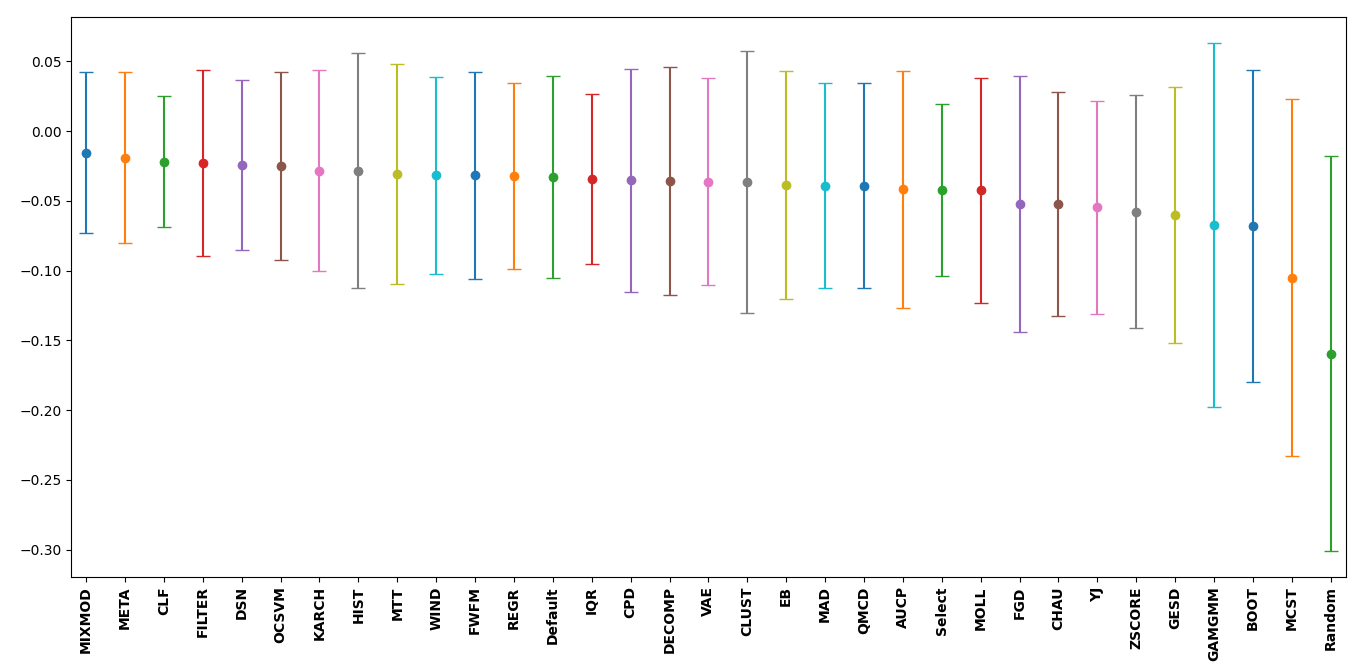
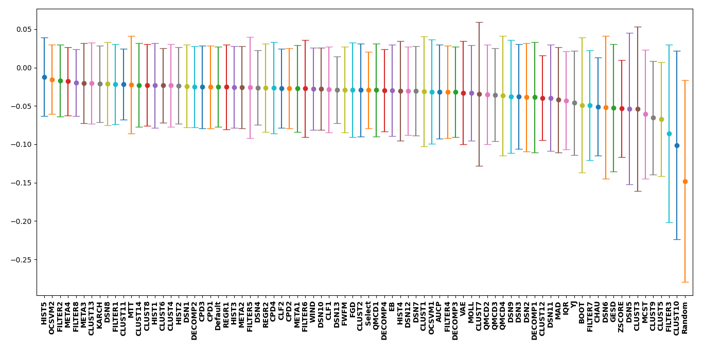
To interpret the plot below, the best to worst performing thresholders have been plotted from left to right with their respective uncertainty. The closer the mean value is to zero, the closer the thresholder performed with regards to the MCC for the labels produced by setting the true contamination level for the selected outlier detection method. However, the uncertainty for many goes beyond zero indicating that in some instances the thresholder performed better than setting true contamination level for a particular dataset and outlier detection method. Along with the thresholders, the default contamination level set for each outlier detection method (Default) = 10% was tested as well as randomly picking a contamination level between 1% - 20% (Select). Finally, a baseline was also calculated if outliers were selected at random (Random). This was done by setting $MCC_{\rm{norm}} = 1$ .

Overall, a significant amount of thresholders performed better than selecting a random contamination level. The MIXMOD thresholder performed best while the CLF thresholder provided the smallest uncertainty about its mean and is the most robust (best least accurate prediction). However, for interpretability and general performance the MIXMOD, FILTER, and META thresholders are good fits.

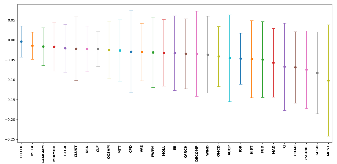
For a deeper look at the different user input parameters for each thresholder, the benchmarking was repeated for the same outlier detection methods as above. However, due to time constraints, only the arrhythmia, cardio, glass, ionosphere, letter, lympho, pima, vertebral, vowels, and wbc datasets were used. The table below indicates the x-axis labels seen in the plot and the thresholding method that it corresponds to. It can be noticed that the best performing thresholder differs from the first plot. This is due to a smaller dataset with fewer examples and a greater bias.

Label	Method
AUCP	AUCP()
BOOT	BOOT()
CHAU	CHAU()
CLF1	CLF(method=’simple’)
CLF2	CLF(method=’complex’)
CLUST1	CLUST(method=’agg’)
CLUST2	CLUST(method=’birch’)
CLUST3	CLUST(method=’bang’)
CLUST4	CLUST(method=’bgm’)
CLUST5	CLUST(method=’bsas’)
CLUST6	CLUST(method=’dbscan’)
CLUST7	CLUST(method=’ema’)
CLUST8	CLUST(method=’kmeans’)
CLUST9	CLUST(method=’mbsas’)
CLUST10	CLUST(method=’mshift’)
CLUST11	CLUST(method=’optics’)
CLUST12	CLUST(method=’somsc’)
CLUST13	CLUST(method=’spec’)
CLUST14	CLUST(method=’xmeans’)
CPD1	CPD(method=’Dynp’)
CPD2	CPD(method=’KernelCPD’)
CPD3	CPD(method=’Binseg’)
CPD4	CPD(method=’BottomUp’)
DECOMP1	DECOMP(method=’NMF’)
DECOMP2	DECOMP(method=’PCA’)
DECOMP3	DECOMP(method=’GRP’)
DECOMP4	DECOMP(method=’SRP’)
DSN1	DSN(metric=’JS’)
DSN2	DSN(metric=’WS’)
DSN3	DSN(metric=’ENG’)
DSN4	DSN(metric=’BHT’)
DSN5	DSN(metric=’HLL’)
DSN6	DSN(metric=’HI’)
DSN7	DSN(metric=’LK’)
DSN8	DSN(metric=’MAH’)
DSN9	DSN(metric=’TMT’)
DSN10	DSN(metric=’RES’)
DSN11	DSN(metric=’KS’)
DSN12	DSN(metric=’INT’)
DSN13	DSN(metric=’MMD’)
EB	EB()
FGD	FGD()
FILTER1	FILTER(method=’gaussian’)
FILTER2	FILTER(method=’savgol’)
FILTER3	FILTER(method=’hilbert’)
FILTER4	FILTER(method=’wiener’)
FILTER5	FILTER(method=’medfilt’)
FILTER6	FILTER(method=’decimate’)
FILTER7	FILTER(method=’detrend’)
FILTER8	FILTER(method=’resample’)
FWFM	FWFM()
GESD	GESD()
HIST1	HIST(method=’otsu’)
HIST2	HIST(method=’yen’)
HIST3	HIST(method=’isodata’)
HIST4	HIST(method=’li’)
HIST5	HIST(method=’triangle’)
IQR	IQR()
KARCH	KARCH()
MAD	MAD()
MCST	MCST()
META1	META(method=’LIN’)
META2	META(method=’GNB’)
META3	META(method=’GNBC’)
META4	META(method=’GNBM’)
MOLL	MOLL()
MTT	MTT()
OCSVM1	OCSVM(model=’poly’)
OCSVM2	OCSVM(model=’sgd’)
QMCD1	QMCD(method=’CD’)
QMCD2	QMCD(method=’WD’)
QMCD3	QMCD(method=’MD’)
QMCD4	QMCD(method=’L2-star’)
REGR1	REGR(method=’siegel’)
REGR2	REGR(method=’theil’)
VAE	VAE()
WIND	WIND()
YJ	YJ()
ZSCORE	ZSCORE()

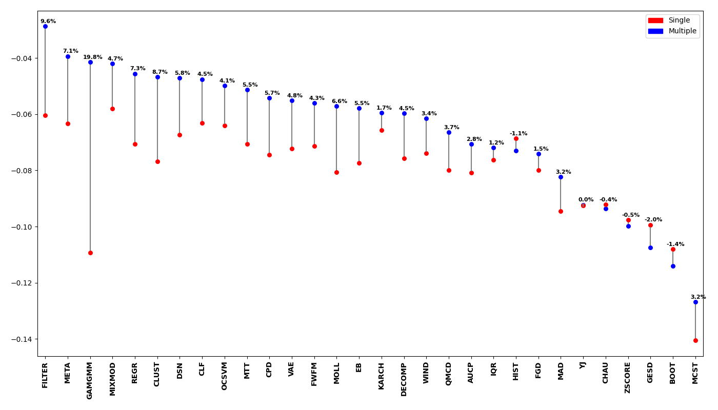
Multiple outlier detection likelihood score sets as of PyThresh version 0.3.3 can now also be thresholded. This functionality is achieved by decomposing the score set using 1D TruncatedSVD decomposition. This allows the decomposed scores to capture a more robust outlier likelihood score set. To benchmark these scores, a similar setup is followed as the first benchmark test, however, the labels were set using the true contamination applied to the decomposed scores as the right-hand component of the MCC deterioration equation.

However, to effectively compare whether the multiple outlier detection likelihood score set performed better than using a single outlier likelihood score set they must both be benchmarked against the same comparison. This can be done by setting the right-hand component of the MCC deterioration to the true labels such that the right-hand component is equal to 1. Below is a vertical dumbbell comparison plot between using single or multiple outlier likelihood score sets for thresholding. Above each comparison a performance percentage indicates how much better or worse multiple scores performed to using single score thresholding. From this, it can be shown that by using a multiple outlier likelihood score set it generally performs better than using a single outlier likelihood scores set.

External Benchmarking

An external benchmark test of all the default thresholders is available in Estimating the Contamination Factor’s Distribution in Unsupervised Anomaly Detection. However it is important to note that a different evaluation metric was used (F1 deterioration), and also since the publishing of this article some default parameters for some thresholders have been changed. Still, this article provides a thorough analysis of the performance of the thresholders in PyThresh with many insightful results and detailed analysis of thresholding outlier decision likelihood scores.

Thresholder Combination

The COMB thresholder allows for combining the output from several thresholders to produce an amalgamated result. However, there are several methods with which to combine thresholders. Each method’s ability to calculate a well-rounded general result from its constituents is important for increased accuracy and overall performance.

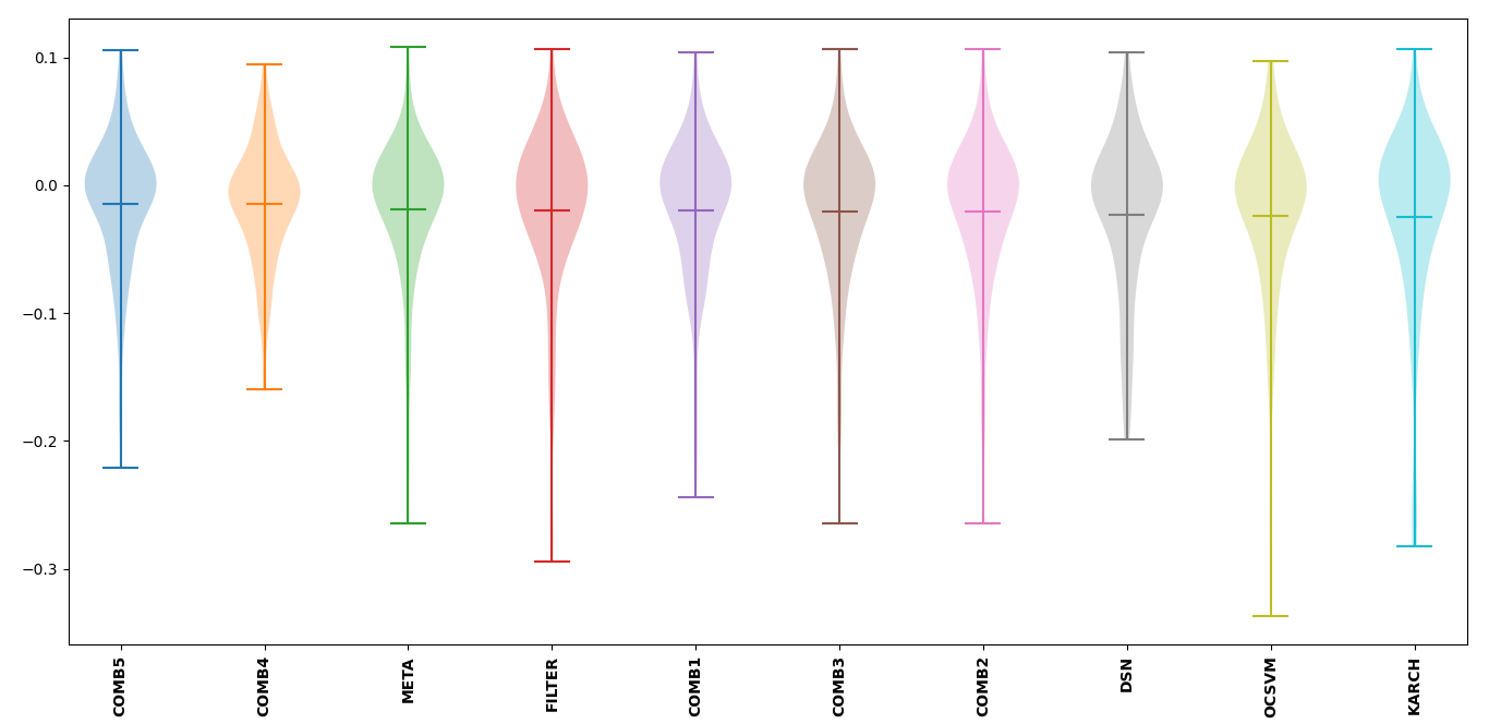
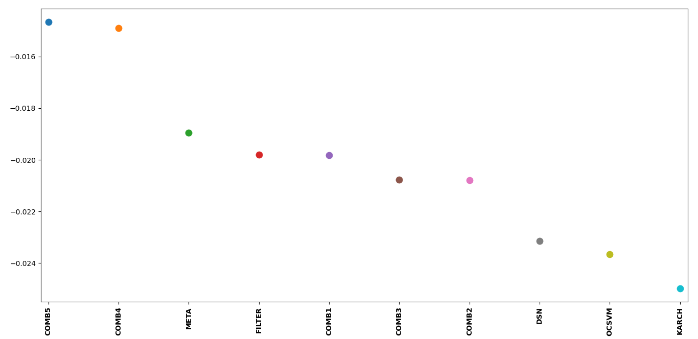
To evaluate the performance of each method available from the COMB thresholder the same outlier detection methods as well as datasets from the first benchmarking test were applied. The selected thresholders that were combined were META, FILTER, DSN, OCSVM, and KARCH all using default parameters. It was found that the bagged and stacked methods performed significantly better than any individual input thresholder while the mean, median, mode methods produced results that were comparable to their inputs.

Label	Method
COMB1	COMB(method=’mean’)
COMB2	COMB(method=’median’)
COMB3	COMB(method=’mode’)
COMB4	COMB(method=’bagged’)
COMB5	COMB(method=’stacked’)

Over Prediction

All thresholders have a tendency to over predict the contamination level of the outlier scores. This will lead to not only mis-classifying inliers based on the outlier detection method’s capabilities but also additional inliers which will lead to a loss of significant data with which to work with. Therefore it is important to note which thresholders have the highest potential to over predict.

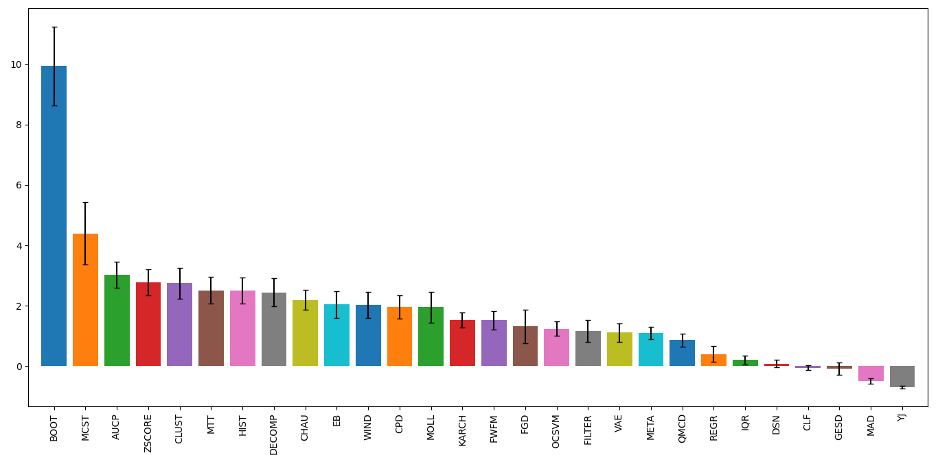
To evaluate the over predictive nature of each thresholder, the ratio between the predicted and true contamination level will be used. The mean of the ratios minus one is calculated for each thresholder using the same setup as the first benchmark test. For this evaluation, a value of 0 indicates perfect contamination predictions, below 0 is under prediction, and above 0 is over prediction. BOOT has the highest potential to over predict while most thresholders in general tend to over predict. It is also important to note that a thresholder’s potential to over predict will vary significantly based on the selected dataset and outlier detection method, and therefore it is important to check the predicted contamination level after thresholding.

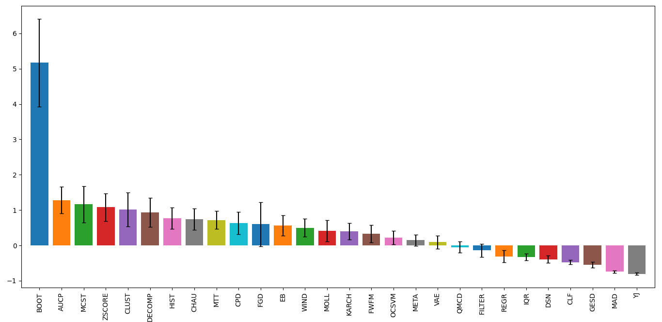
A second over predictive evaluation can also be done, but now with regards to over predicting beyond the best contamination level for each outlier detection method on each dataset based on the MCC score. As seen below, a significant amount of thresholders still tend to over predict even beyond the best contamination level. However, now some clear well performing thresholders can be matched to the previous benchmarking, notably META and FILTER.

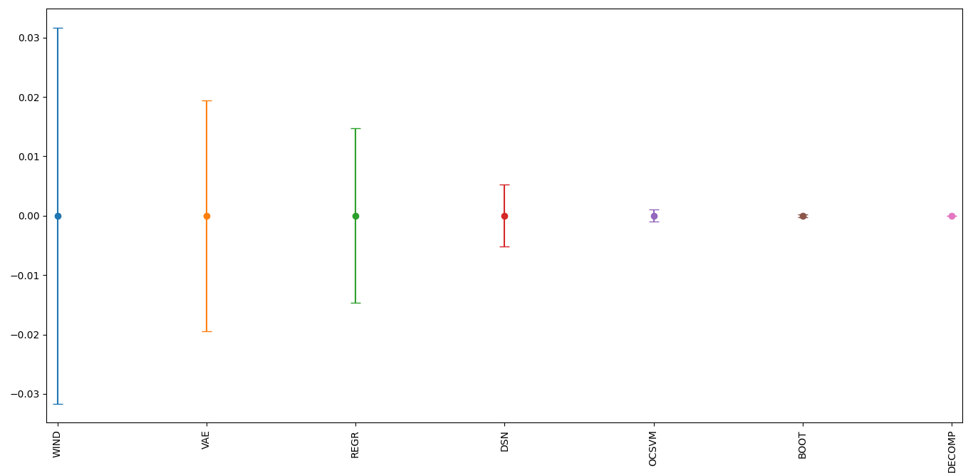
Effects of Randomness

Some thresholders use randomness in their methods and the random seed can be set using the parameter random_state. To investigate the effect of randomness on the resulting labels the MCC deterioration was calculated for each thresholder using the random states (1234, 42, 9685, and 111222). The same outlier detection methods as well as datasets from the first benchmarking test were applied. The means of the MCC deterioration were normalized to zero showing the extent of the effect of randomness of each thresholder’s ability to evaluate labels for the outlier decision likelihood scores indicated in the uncertainty.

From the plot below, WIND performed the worst and was highly affected by the choice of the selected random state. DSN which is a thresholder that overall performed well during the benchmark tests is also sensitive to randomness. To alleviate the effects of randomness on the thresholders, it is recommended that a combined method be used by setting different random states (e.g. COMB(thresholders = [DSN(random_state=1234), DSN(random_state=42), DSN(random_state=9685), DSN(random_state=111222)])). This should provide a more robust and reliable result.

Time Complexity

Working with big data can mean time constraints with regards to thresholding. Therefore, time complexity may need to be considered when selecting the correct thresholder to use. This time complexity can be quantified by using the Big-O notation metric. This metric demonstrates how many seconds it takes to compute the number of outlier likelihood scores (n). From the benchmark table below, it can be seen that most thresholders have a quadratic time complexity of around ~1e-8*n^2. This is due to most thresholders using kernel density estimations within their methods. This time complexity equates about 0.01s for 1000 datapoints, 1s for 10000 datapoints, 100s for 100000 datapoints, and about 2.5 hours for 1 million datapoints. If time is a factor, suggested thresholders with reasonable accuracy are: FILTER with 10s, OCSVM with 0.1s, and MTT with 100s for one million datapoints. Note that these benchmarks were done using an i5 12th gen processor and results may scale slightly differently depending on the hardware used.

Method	Complexity	Big-O Notation
AUCP	Quadratic	~1e-8*n^2
BOOT	Quadratic	~1e-8*n^2
CHAU	Linear	~1e-8*n
CLF	Quadratic	~1e-8*n^2
CLUST	Quadratic	~1e-8*n^2
CPD	Quadratic	~1e-8*n^2
DECOMP	Quadratic	~1e-8*n^2
DSN	Quadratic	~1e-8*n^2
EB	Linearithmic	~1-06nlog(n)
FGD	Quadratic	~1e-8*n^2
FILTER	Quadratic	~1e-11*n^2
FWFM	Quadratic	~1e-8*n^2
GAMGMM	Quadratic	~1e-6*n^2
GESD	Quadratic	~1e-9*n^2
HIST	Linear	~1e-8*n
IQR	Linear	~1e-8*n
KARCH	Quadratic	~1e-8*n^2
MAD	Linear	~1e-8*n
MCST	Quadratic	~1e-7*n^2
META	Cubic	~1e-12*n^3
MIXMOD	Linear	~1e-4*n
MOLL	Quadratic	~1e-10*n^2
MTT	Quadratic	~1e-10*n^2
OCSVM	Linear	~1e-7*n
QMCD	Quadratic	~1e-9*n^2
REGR	Quadratic	~1e-8*n^2
VAE	Linear	~1e-3*n
WIND	Quadratic	~1e-8*n^2
YJ	Quadratic	~1e-8*n^2
ZSCORE	Linear	~1e-8*n