Thresholding Confidence

Introduction

When thresholding outlier likelihood scores, we obtain a binary array of thresholded labels that categorize data points as either inliers or outliers. However, to confidently assess whether these thresholded labels are within an acceptable range of thresholding confidence for their assignments, a statistical approach is required.

There are various methods to approach this, and one such method involves the use of t-test confidence intervals. A t-test is a statistical test used to compare the means of a sample or two groups of samples. It serves as a hypothesis test to determine whether a point within a sample or two groups of samples differs significantly from one another and quantifies this difference. A confidence interval refers to the probability that a population parameter will fall within a set of values for a certain proportion of times. These confidence intervals can be employed to evaluate whether a data point falls within or outside a specific level of confidence in a sample’s distribution. This clear boundary can help determine if a data point is statistically significant in its assigned label.

In the context of outlier detection thresholding, this ‘sample’ refers to the assigned label and can be used to quantify, with a selected degree of confidence, whether the assigned label is statistically significant. If a data point falls outside this confidence interval, it suggests that the data point is more accurately attributed to a new label, signifying uncertainty regarding its status as an inlier or outlier

In order to determine this thresholding confidence for thresholding outlier detection likelihood scores as mentioned above, the CONF utility in pythresh.utils.conf has been specifically written for this purpose.

Methodology

Before jumping into how the thresholding confidence is calculated, it is important to note that PyThresh essentially has two fundamental types of thresholding methods. First, are methods that have precise points within the outlier likelihood scores where a threshold point is set. These methods can be referred to as continuous based methods. The other thresholding methods rather define inliers and outlier based on some classification type criterion and therefore possess no defined threshold point. These methods can be referred to as classification based methods.

Continuous Based

For continuous based thresholding methods, the thresholding confidence is calculated as follows:

All the outlier likelihood scores are thresholded and the .thresh_ attribute is calculated
A sample of outlier likelihood scores is selected.
The chosen thresholding method is then applied to this sample.
The .thresh_ attribute of an evaluated thresholder is then stored, defining the boundary from the sample that defines inliers from outliers.
The above three processes are repeated based on the number of chosen tests and each boundary value is stored.
This stored list of boundaries now contains a distribution of boundary points for the selected thresholder.
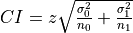
The upper and lower confidence intervals of this distribution can be calculated using the confidence interval equation for a sample given by $CI = z \frac{\sigma}{\sqrt{n}}$ where $z, \sigma, n$ the t-distribution critical value for a selected confidence level for a sample size, the standard deviation of the distribution, and the number of datapoints within the sample respectively.
With the lower and upper confidence intervals, outlier likelihood scores that fall within the threshold bound with regards to all the outlier likelihood scores .thresh_ $\pm CI$ are then set as uncertains and their indeces are returned.

Classification Based

For classification based thresholding methods, the thresholding confidence is calculated as follows:

All the outlier likelihood scores are thresholded and their binary labels are stored
A sample of outlier likelihood scores is selected from a stratified list of the above labels.
The chosen thresholding method is then applied to this sample.
The new labels for this sample is stored
The above three processes are repeated based on the number of chosen tests sample labels are stored.
Using the stored 2D array of labels, the ratio for each datapoint based on the number of times it was classed the same as the binary labels for the whole dataset versus the total number of tests is calculated.
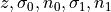From this a two independent sample confidence interval test can be calculated using $CI = z \sqrt{\frac{\sigma_{0}^2}{n_0} + \frac{\sigma_{1}^2}{n_1}}$ where $z, \sigma_0, n_0, \sigma_1, n_1$ are the t-distribution critical value for a selected confidence level for the combined sample size, the standard deviation of the sample for the inlier label ratios, the sample size of the inliers, the standard deviation of the sample for the outlier ratios, and the sample size of the outliers respectively.
With the lower and upper confidence intervals, inlier labels ratios that lie beyond the mean of the inlier ratio plus $CI$ , and outlier labels ratios that lie beyond the mean of the outlier ratio minus $CI$ are then set as uncertains and their indeces are returned.

Example

Below is a simple example of how to apply the CONF method for the musk dataset:

import os

import numpy as np
from pyod.models.iforest import IForest
from pyod.utils.utility import standardizer
from pythresh.thresholds.clf import CLF
from pythresh.thresholds.iqr import IQR
from pythresh.utils.conf import CONF
from scipy.io import loadmat
from sklearn.decomposition import PCA


mat_file = 'musk.mat'

mat = loadmat(os.path.join('data', mat_file))

X = mat['X']
y = mat['y'].ravel()

X = standardizer(X)

clf = IForest(random_state=1234)
clf.fit(X)

scores = clf.decision_scores_

thres = IQR()
labels = thres.eval(scores)

confidence = CONF(thres, alpha=0.05, split=0.2)
unc_idx = confidence.eval(scores)

decomp = PCA(n_components=2, random_state=1234)
X = decomp.fit_transform(X)

uncertain = X[unc_idx]
ouliers = X[labels==1]
inliers = X[labels==0]

fig = plt.figure(figsize=(18, 12))
plt.plot(inliers[:, 0], inliers[:, 1], 'y.', label='Inliers', markersize=10)
plt.plot(outliers[:, 0], outliers[:, 1], 'r.', label='Outliers', markersize=11)
plt.plot(uncertains[:, 0], uncertains[:, 1], 'b.', label='Uncertains', markersize=12)
plt.legend()
plt.show()

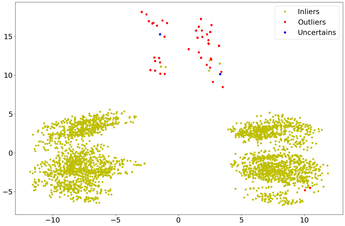
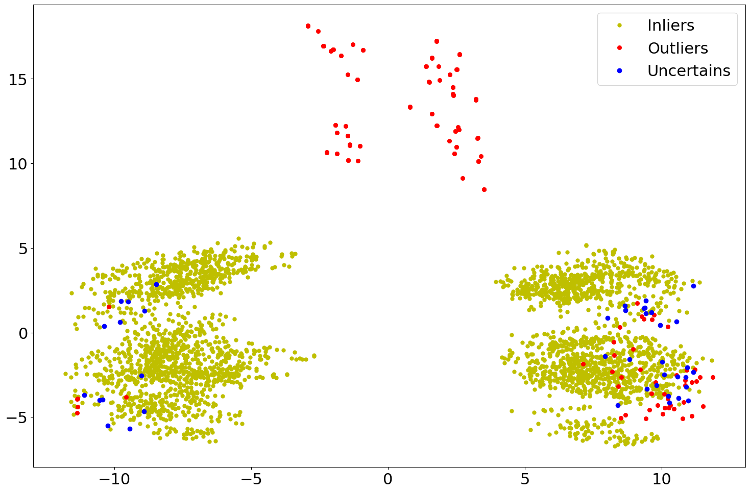
Below are two scatter plots of the results from the example code above. However, in the second plot the use of a classification type thresholder CLF has been employed.

Scatter plot of the above example 1 — Figure 1: Scatter plot of the `CONF` evaluated results using `IQR`.

Scatter plot of the above example 2 — Figure 2: Scatter plot of the `CONF` evaluated results using `CLF`.