Ranking
Introduction
Outlier detection for unsupervised tasks is difficult. The difficulty arises with how to evaluate whether the selected methods for outlier detection and thresholding are correct or the best for the dataset. Often, additional post-evaluation involves visual or domain knowledge based decisions to make a final call. This process can be tedious and is often just as complex as the methods used to do the outlier detection in the first place.
However, there are some robust statistical methods that can be used to indicate or at least provide a guide of which outlier detection and thresholding methods perform better than others. This process is that of a ranking problem and can be used to list in order the evaluated outlier detection and thresholding methods in terms of their respective performance with other methods.
In order to rank the multiple outlier detection and thresholding methods’ capabilities of effectively labeling a given dataset, it is important to note what is defined by “capabilities”. In this case, this refers to how well the predicted labels solved by the outlier detection and thresholding method compares to the true labels. This can be done using the F1 score or Matthews correlation coefficient (MCC). But, since unsupervised tasks means there is lack of true labels, the best option is to use other robust statistical metrics that have a strong correlation to the above mentioned scores.
To find these proxy-metrics a good starting point is to know what data can be used to compute them. In the case of unsupervised outlier detection, there are essentially three main components: the exploratory variables (X), the predicted outlier likelihood scores, and the thresholded binary labels. With these, criteria can be set to apply proxy-metrics that can then be ranked to provide a list of best to worst performing outlier detection and thresholding methods with respect to these metrics.
Proxy-Metrics
Different types of proxy-metrics can be used with respect to the F1 and MCC. Below four catagories have been defined.
Clustering Based
Since the dataset is considered to contain outliers, a clear distinction should exist between the inliers and outliers. By using clustering based metrics, the measure of similarity or distance between centroids or each datapoints can provide a single score of outlier detection method’s to effectively distinguish inliers from outliers. This should also indicate greater distinction between the inlier and outlier clusters. For these clustering based metrics the quality of the labeled data will be evaluated using either the exploratory variables or the outlier likelihood scores and their assigned labels Automatic Selection of Outlier Detection Techniques
Statistical Distances
Statistical distances quantify the measure of distances between probability based measures. These distances can be used to compute a single value difference between two probability distributions. This hints to what data from the unsupervised outlier detection method task should be used. Two distinct probability distributions can be computed for the outlier likelihood scores with respected to their labeled class.
Curve Based
Curve based method like clustering based methods can be used to compare the performance of unsupervised anomaly detection algorithms. This is done by leveraging the density of OD likelihood scores and evaluating their distributions with particular interest on their tails as this is typically where the outlier will lie How to Evaluate the Quality of Unsupervised Anomaly Detection Algorithms?
Consensus Based
Since the other proxy-metrics evaluate each outlier detection method individually, consensus based proxy-metrics rather compare the OD methods against one another. This is done be creating a consensus baseline by using all the OD method’s results and comparing the deviation of each OD method from this baseline. This allows for a consensus based score to be assigned to each OD method with respect to the other tested OD methods A Large-scale Study on Unsupervised Outlier Model Selection: Do Internal Strategies Suffice? Consensus outlier detection in survival analysis using the rank product test
Proxy-Metrics Correlation Tests
35 proxy-metrics scores were correlated against the true versus the
thresholded labels MCC score by applying Pearson’s correlation. This was
done for all passing possible combinations of the PyOD outlier
detection methods LODA, QMCD, MCD, GMM, KNN, KDE, PCA, COPOD, HBOS,
and IForest on the AD benchmark datasets: annthyroid, breastw,
cardio, Cardiotocography, fault, glass, Hepatitis, Ionosphere, landsat,
letter, Lymphography, mnist, musk, optdigits, PageBlocks, pendigits,
Pima, satellite, satimage-2, SpamBase, Stamps, thyroid, vertebral,
vowels, Waveform, WBC, WDBC, Wilt, wine, WPBC, and yeast available
at ADBench dataset
and applying the FILTER, CLF, DSN, OCSVM, KARCH, HIST, and META
thresholders. A total of 198357 possible passing (dropped error fits,
nans, and infs) combinations were tested for this evaluation. Tabulated
below is a meta-analysis of the proxy-metrics Pearson’s score statistics
calculated for all the combination across the datasets.
For clustering based between the exploratory variables and the predicted labels, the following proxy-metrics were tested.
CAL: Calinski-Harabasz
DAV: Davies-Bouldin score
SIL: Silhouette score
For clustering based between the outlier likelihood scores and the predicted labels, the following proxy-metrics were tested.
BH: Ball-Hall Index
BR: Banfeld-Raftery
CAL_sc: Calinski-Harabasz score
DAV_sc: Davies-Bouldin score
DR: Det Ratio Index Dunn: Dunn’s index
Hubert: Hubert index
Iind: Local Moran’s I index
MR: Mclain Rao Index
PB: Point biserial Index
RL: Ratkowsky Lance Index
RT: Ray-Turi Index
SIL_sc: Silhouette score
SDBW: S_Dbw validity index
SS: Scott-Symons Index
WG: Wemmert-Gancarski Index
XBS: Xie-Beni index
For statistical distances, the following proxy-metrics were tested.
AMA: Amari distance
BHT: Bhattacharyya distance
BREG: Exponential Euclidean Bregman distance
COR: Correlation distance
ENG: Energy distance
JS: Jensen-Shannon distance
MAH: Mahalanobis distance
LK: Lukaszyk-Karmowski metric for normal distributions
WS: Wasserstein or Earth Movers distance
For curve based, the following proxy-metrics were tested.
EM: Excess-Mass curves
MV: Mass-Volume curves
For consensus based, the following proxy-metrics were tested.
Contam: Mean contamination deviation based on TruncatedSVD decomposed scores
GNB: Gaussian Naive-Bayes trained consensus score
HITS: Deviation from the HITS consensus authority based labels
Mode: Deviation from the mode of the predicted labels
Thresh: Label deviation from the TruncatedSVD decomposed thresholded labels
Label |
Mean |
Median |
Standard Deviation |
|---|---|---|---|
CAL |
0.1872 |
0.2027 |
0.4303 |
DAV |
-0.1257 |
-0.0474 |
0.4523 |
SIL |
0.1262 |
0.0589 |
0.4744 |
BH |
0.0039 |
0.0391 |
0.4836 |
BR |
0.0260 |
0.0300 |
0.4750 |
CAL_sc |
0.0158 |
0.0111 |
0.5083 |
DAV_sc |
-0.0483 |
-0.0944 |
0.5230 |
DR |
-0.0157 |
-0.0111 |
0.5084 |
Dunn |
0.0270 |
0.0207 |
0.5353 |
Hubert |
0.0641 |
0.1632 |
0.4674 |
Iind |
0.0648 |
0.1527 |
0.4763 |
MR |
0.0789 |
0.1710 |
0.4973 |
PB |
0.0367 |
0.0715 |
0.5089 |
RL |
-0.0314 |
-0.0569 |
0.5081 |
RT |
-0.0034 |
0.0524 |
0.4884 |
SIL_sc |
0.0473 |
0.0801 |
0.4885 |
SDBW |
-0.0641 |
-0.0627 |
0.4736 |
SS |
-0.0034 |
0.0524 |
0.4884 |
WG |
-0.0244 |
-0.0210 |
0.5221 |
XBS |
-0.0535 |
0.0032 |
0.5280 |
AMA |
0.0543 |
0.0088 |
0.5046 |
BHT |
0.0239 |
0.0163 |
0.5050 |
BREG |
0.1022 |
0.1546 |
0.5006 |
COR |
0.0173 |
0.0364 |
0.5114 |
ENG |
0.1120 |
0.1054 |
0.5030 |
JS |
0.0566 |
0.1282 |
0.5045 |
MAH |
0.0749 |
0.0300 |
0.5075 |
LK |
0.0749 |
0.1048 |
0.5070 |
WS |
0.1133 |
0.1766 |
0.5001 |
EM |
0.0261 |
0.0752 |
0.4332 |
MV |
0.0094 |
-0.0164 |
0.4361 |
Contam |
-0.2003 |
-0.1498 |
0.5297 |
GNB |
-0.1931 |
-0.2902 |
0.4768 |
HITS |
-0.0449 |
-0.1235 |
0.5998 |
Mode |
-0.1505 |
-0.0840 |
0.5377 |
Thresh |
-0.1696 |
-0.1940 |
0.6031 |
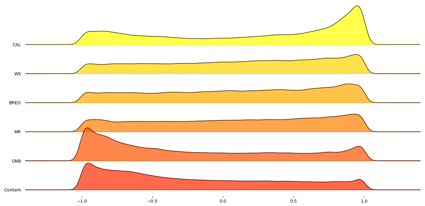
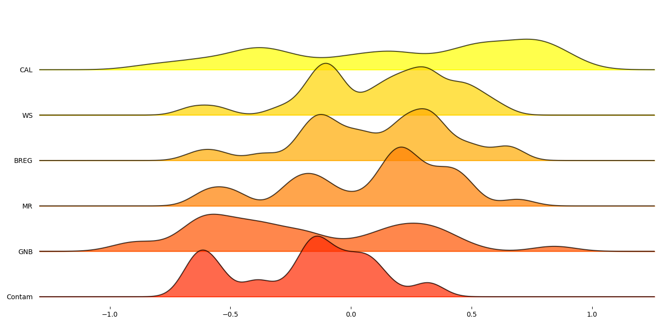
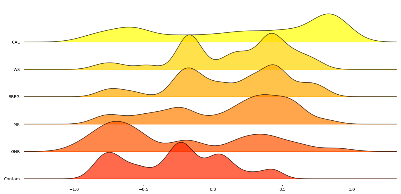
From the table above it can be seen that most proxy-metrics performed sub-optimally. However, there were six proxy-metrics that performed generally better than the others. These are the six proxy-metrics
The Calinski-Harabasz score
The Mclain Rao Index
The Exponential Euclidean Bregman distance
The Wasserstein distance
The mean contamination deviation based on TruncatedSVD decomposed scores
The Gaussian Naive-Bayes trained consensus score
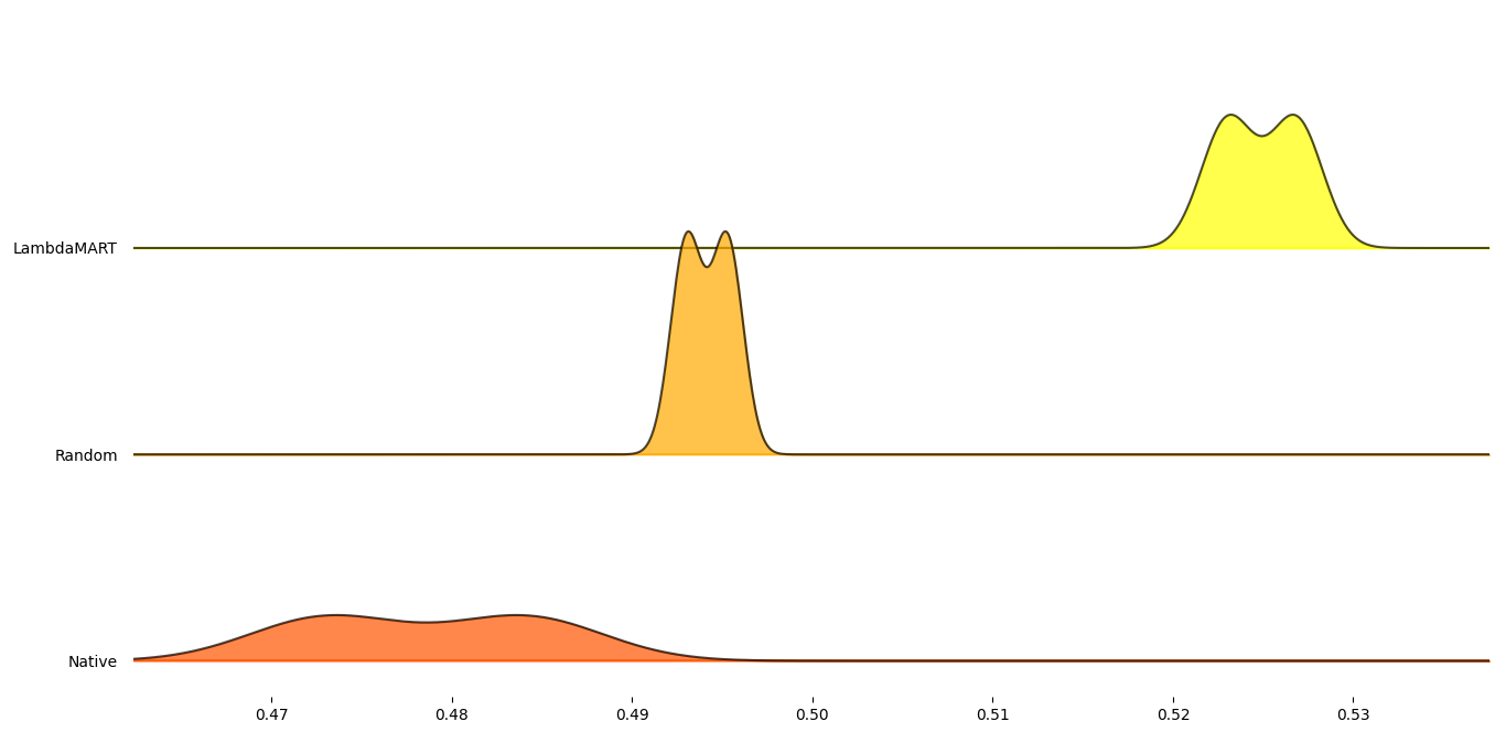
In order to get a better understanding on how these six proxy-metrics performed overall, joyplots below demonstrate the distributions of their Pearson’s correlation with respect to the MCC scores for each statistic.
Rank OD Methods
The ranking process involves ordering the proxy-metric scores with respect to their performance. The proxy-metrics are ordered highest-to-lowest or lowest-to-highest based on their performance criterion. The proxy-metrics are combined as follows: the statistical based distances are combined using equal weighting on their ordered ranks to compute a single ranked list. The same method is applied to the clustering based, and consensus based metrics. Finally, an overall combined rank is computed using the combined statistical based ranking, the combined clustering based ranking, and the combined consensus based ranking. This final combined ranking can either be computed using equal weightings for each three combined rankings or a weight list can be parsed based on preference.
The RANK method in PyThresh applies the method above to rank the
performance of the outlier detection and thresholding methods against
each other.
To evaluate the performance of RANK the ranking evaluation measure
was employed as described in RankDCG: Rank-Ordering Evaluation Measure and GitHub implementation ranking
The RANK method was tested on the same dataset and OD and
thresholding methods as was used for the selected proxy-metrics.
Additionally, a fine-tuned LambdaMART model using XGBoost was also
trained on the selected proxy-metrics and ranks from the same dataset
with which to further evaluate the RANK performance. Also a random
ordered selection rank method was tested with which to compare the
RankDCG results to.
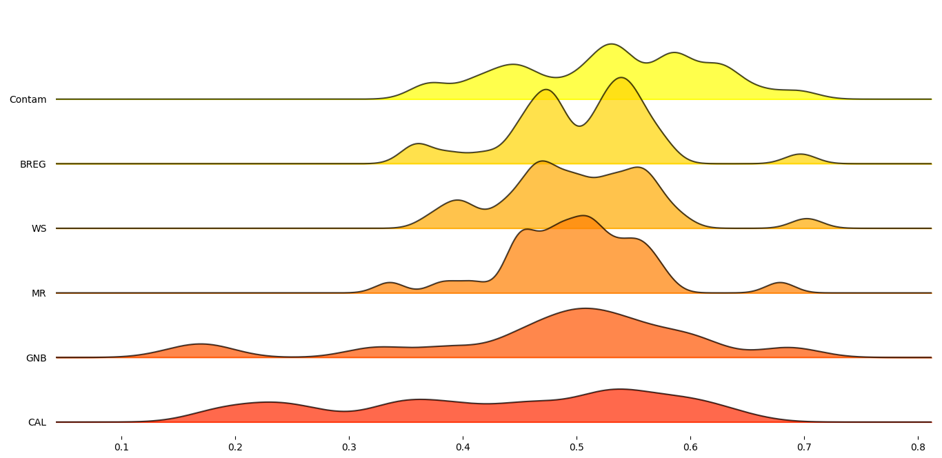
The joyplots below indicate the performance between the methods with respect aggregation across each dataset.
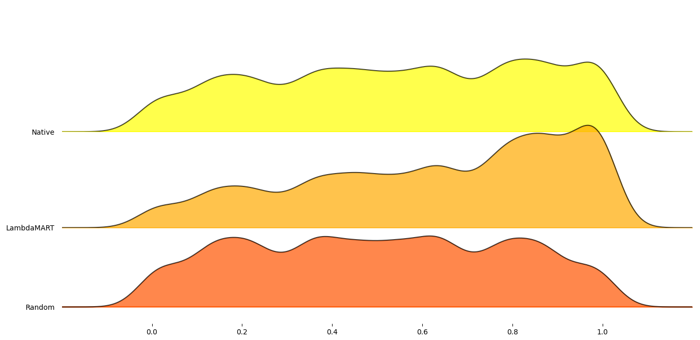
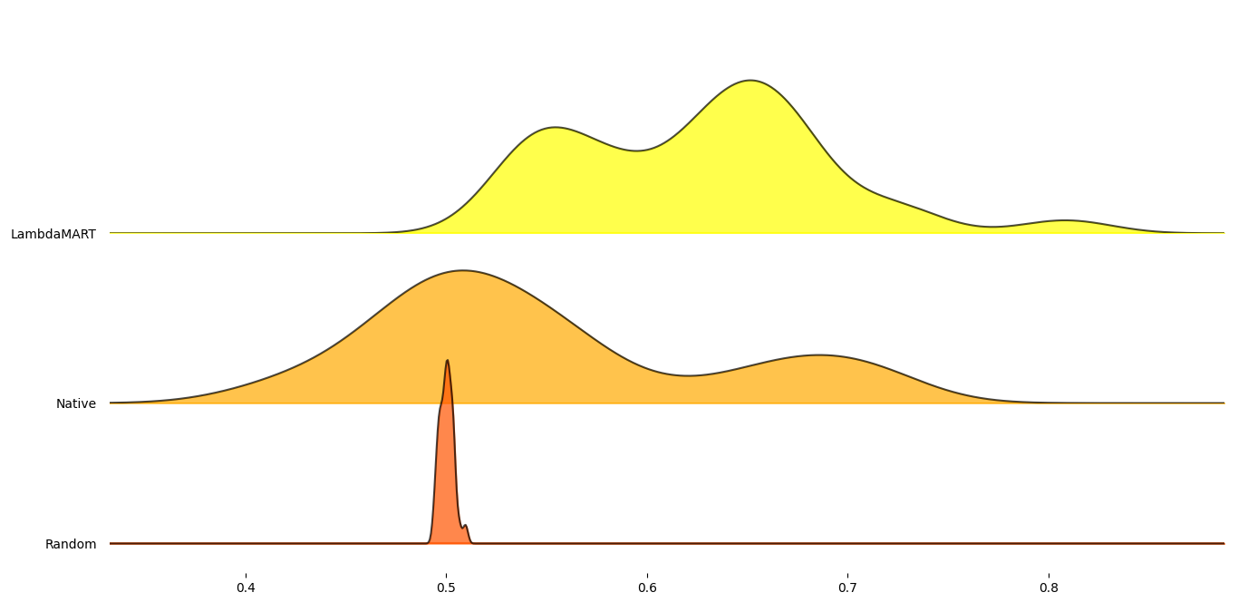
As can be seen, the RANK method performed on average better than
random selection. However, the trained LambdaMART model achieved
significantly better scores than RANK. To test that the model was
not overfitted and is able to generalize, the datasets mammography,
skin, and smtp were tested as the model had not been trained on
them.
On these datasets the RANK method performed worse than random
selection. However, the trained LambdaMART model performed marginally
better than random selection. The lower performance of the model may be
due to the proxy-metrics’ lower than training datasets correlation to
the MCC as well as the OD and thresholding methods performing poorly in
general on these dataset. This is reiterated as seen by the RANK
method’s performance. However, the model is still valid with respect to
its ability to rank OD and thresholding problems.
Example
Below is a simple example of how to apply the RANK method:
# Import libraries
from pyod.models.knn import KNN
from pyod.models.iforest import IForest
from pyod.models.pca import PCA
from pyod.models.mcd import MCD
from pyod.models.qmcd import QMCD
from pythresh.thresholds.filter import FILTER
from pythresh.utils.rank import RANK

# Initialize models
clfs = [KNN(), IForest(), PCA(), MCD(), QMCD()]
thres = FILTER() # or list of thresholder methods

# Get rankings
ranker = RANK(clfs, thres)
rankings = ranker.eval(X)
Final Notes
While the RANK method is a useful tool to assist in selecting the
possible best outlier detection and thresholding method to use, it is
not infallible. The use of the trained LambdaMART model will be used by
default however the standard RANK method can also be employed. It
has been noted from the tests above, that in general the ranked results
tended to return the best-to-worst performing outlier detection and
thresholding methods in the correct order. However, they were not
perfect. They at times exhibited incorrect orders and often the best
performing OD and thresholding method was in the top three rather than
being the top of the list. Additionally, some times well performing OD
and thresholding methods was ranked poorly.
Future work will test to see how effective this method is with regards
to other ranking OD and thresholding methods as well as how much better
it performs than simply picking the IForest OD method.
Note that this method is under active development and the model and methods will be updated or upgraded in the future
The RANK method should be used with discretion but hopefully provide
more clarity on which OD and thresholding method to select.